17. Extended Kalman Filter
Extended Kalman Filter
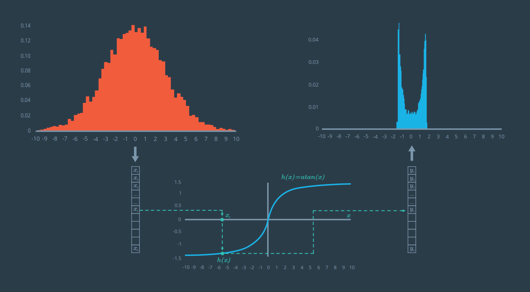
Follow the arrows from top left to bottom to top right: (1) A Gaussian from 10,000 random values in a normal distribution with a mean of 0. (2) Using a nonlinear function, arctan, to transform each value. (3) The resulting distribution.
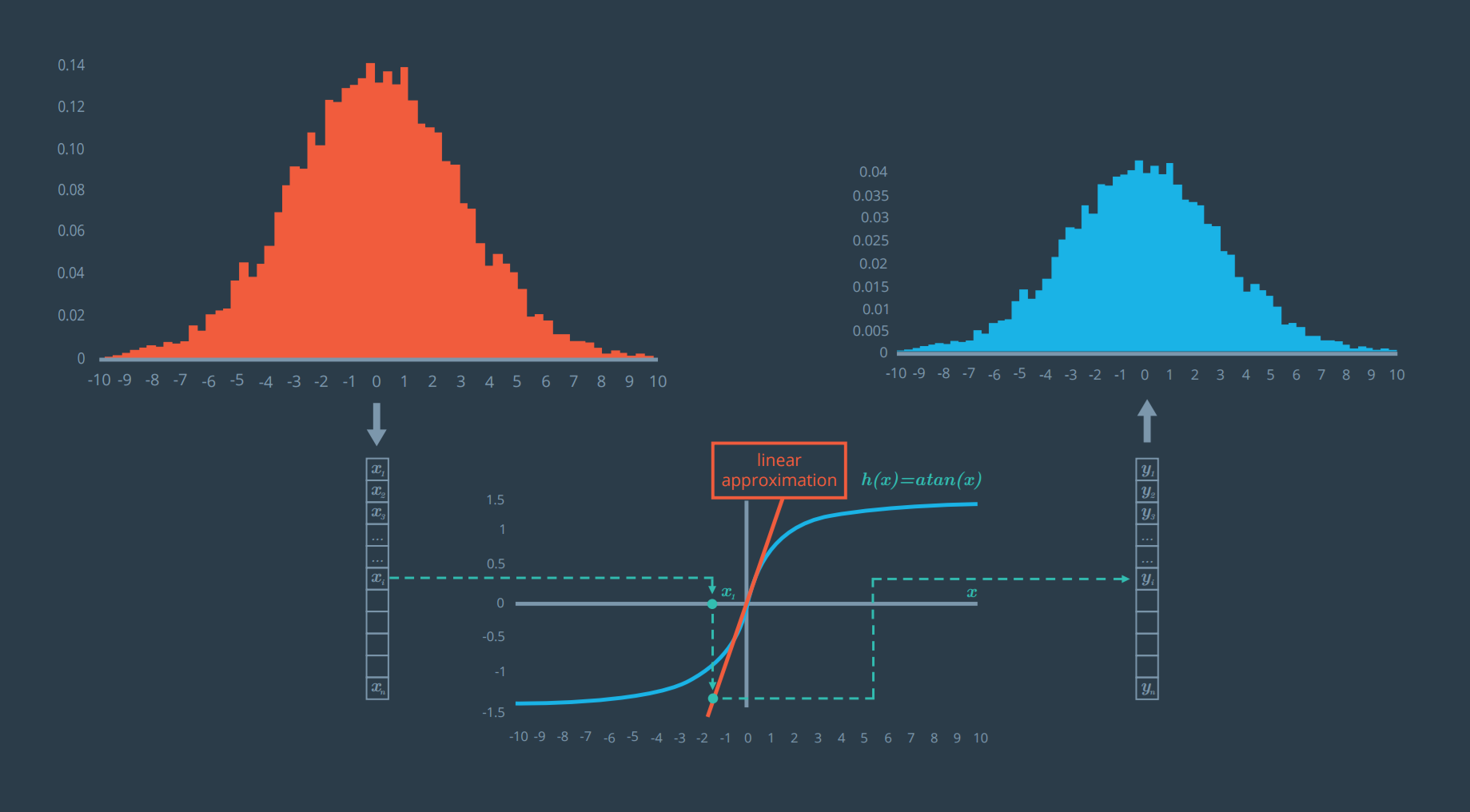
This one looks much better! Notice how the blue graph, the output, remains a Gaussian after applying a first order Taylor expansion.
How to Perform a Taylor Expansion
The general form of a Taylor series expansion of an equation, f(x) , at point \mu is as follows:
f(x) \approx f(\mu) + \frac{\partial f(\mu)}{\partial x} ( x - \mu)
Simply replace f(x) with a given equation, find the partial derivative, and plug in the value \mu to find the Taylor expansion at that value of \mu .
See if you can find the Taylor expansion of arctan(x) .
Let’s say we have a predicted state density described by
\mu = 0 and \sigma = 3 .
The function that projects the predicted state, x , to the measurement space z is
h(x) = arctan(x) .
and its partial derivative is
\partial h = 1/(1+ x^2) .
I want you to use the first order Taylor expansion to construct a linear approximation of h(x) to find the equation of the line that linearizes the function h(x) at the mean location \mu .
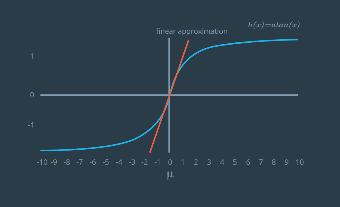
The orange line represents the first order Taylor expansion of arctan(x). What is it?
A) h(x) \approx x
B) h(x) \approx 1/(1+x^2)
C) h(x) \approx x + arctan(x)
D) h(x) \approx 3 + x